Quick Start Guide

This chapter shows a simple example of how to use ORBKIT. Here, we compute four molecular orbitals (HOMO-1, HOMO, LUMO, and LUMO+1) of a water molecule and we demonstrate its quick visualization with VMD and Mayavi. The execution is demonstrated within the Terminal and within a Python shell.

Note

We assume that you have followed the Installation Instructions and that you have navigated to the folder $ORBKITPATH/examples/basic_examples. For reasons of clarity, we write all output in a subfolder named vis:

$ cd $ORBKITPATH/examples/basic_examples
$ mkdir vis

Within the Terminal

Using VMD

The fastest and easiest way of preparing good-looking depictions of molecular orbitals or the electron density is by creating cube files and a VMD script. For non-commercial use, VMD is a free program.

Now, let us run ORBKIT for a grid adapted to the molecular geometry (see Grid Related Options for details):

$ orbkit -i h2o.molden -o vis/h2o --otype=vmd --adjust_grid=5 0.5 --calc_mo=homo-1:lumo+2

ORBKIT creates four cube files and a VMD script file vis/h2o_MO.vmd. This can be displayed using VMD by calling

$ vmd -e vis/h2o_MO.vmd

By default, ORBKIT uses absolute paths within the VMD script file.

Hint

The orbital numbering corresponds to the indices within the input file (counting from one!). When you select a range of orbitals using a colon “:”, please note that we are using the syntax of the Python range function, i.e., --calc_mo=START:STOP[:STEP], where STOP is not an element of the list.

Using Mayavi

To get a rough overview over the shape of the quantities computed, you can use a simple interface to Mayavi. Although, no output file is created with that option, you can combine it with other output options, e.g., --otype=vmd.

Now, let us run ORBKIT for a grid adapted to the molecular geometry (see Grid Related Options for details):

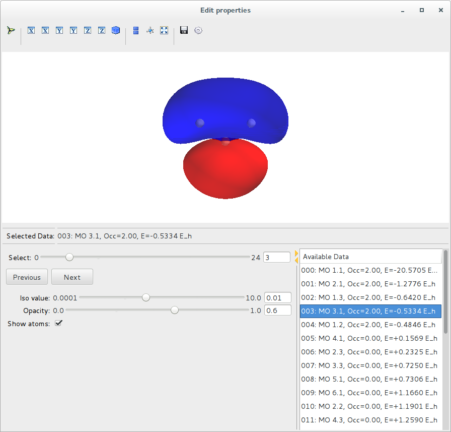
$ orbkit -i h2o.molden --otype=mayavi --adjust_grid=5 0.5 --calc_mo=homo-1:lumo+2

When the computations are finished, the data will be depicted in an interactive window:

Within a Python Shell

All tasks mentioned above can be directly performed within a Python shell. This will be shown in the following, i.e., we will compute a set of molecular orbitals on a grid adjusted to the molecular geometry, and for the depiction, we will create both, a VMD script and a Mayavi scene.

Using ORBKIT’s High-Level Interface

First, import the required python modules:

>> from orbkit import options, main

Set the options

>> options.filename = 'h2o.molden'
>> options.outputname = 'vis/h2o'
>> options.otype = ['vmd','mayavi']
>> options.adjust_grid = [5,0.1]
>> options.calc_mo = 'homo-1:lumo+2'

and run ORBKIT.

>> mo_list, mo_info = main.run_orbkit()

Using ORBKIT’s Low-Level Interface

This task can also be accomplish by using the respective functions directly. First, import the required python modules:

>> from orbkit import read, grid, extras, output, display

Read the input file,

>> qc = read.main_read('h2o.molden',itype='molden',all_mo=True)

initialize the grid,

>> grid.adjust_to_geo(qc,extend=5.0,step=0.1)
>> grid.grid_init()
>> display.display(grid.get_grid())

and run the calculation (incl. storage of the output)

>> mo_list, mo_info = extras.calc_mo(qc,'homo-1:lumo+2',otype=['vmd','mayavi'],ofid='vis/mo')

If you want to compute and depict other quantities than molecular orbitals, you can choose between orbkit.core.rho_compute or orbkit.extras.mo_set. When you use orbkit.core.rho_compute directly, you have to create the output by your own:

>> from orbkit import output
>> output.main_output(mo_list,qc.geo_info,qc.geo_spec,outputname='vis/mo',otype=['vmd','mayavi'])