Tutorial for Processing Multiple Input Files

We assume that you have followed the Installation Instructions and that you have navigated to the folder $ORBKITPATH/examples/basic_examples. The input files you will need for this tutorial are compressed in .tar.gz file in the examples folder ($ORBKITPATH/examples/basic_examples/NaCl_molden_files.tar.gz). There is no need to extract the files as ORBKIT is able to read them directly from the .tar.gz archive.

Hint

This tutorial explains parts of the example file $ORBKITPATH/examples/basic_examples/use_for_ordering.py.

How to Read a List of Files

As a starting point, you have to import the ORBKIT module for processing multiple files:

from orbkit import multiple_files

The input files can then be read with:

multiple_files.read('NaCl_molden_files.tar.gz',all_mo=True,nosym=False)

Now, all input variables are global values in the module multiple_files. These variables are named according to their analogue in the QCinfo class (cf. Central Variables):

Variable	Contents
geo_spec_all	Contains all molecular geometries, see geo_spec in Central Variables.
geo_info	See geo_info in Central Variables.
ao_spec	See ao_spec in Central Variables.
mo_coeff_all	Contains all molecular orbital coefficients. List of numpy.ndarray.
mo_energy_all	Contains all molecular orbital energies. List of numpy.ndarray.
mo_occ_all	Contains all molecular orbital occupations. List of numpy.ndarray.
sym	Python dictionary containing the molecular orbital symmetries and the corresponding position in mo_coeff_all, mo_energy_all, and mo_occ_all, respectively.
index_list	After the execution of the ordering routine, it contains the new indices of the molecular orbitals. If index < 0, the molecular orbital changes its sign. shape=(Nfiles,NMO).

How to Order the Molecular Orbital Coefficients

ORBKIT provides different schemes to order molecular orbitals, of which the best shall be presented here: the ordering using analytical integrals between neighboring molecular orbitals.

This procedure is a black box procedure and can be called with:

index_list, mo_overlap = multiple_files.order_using_analytical_overlap(None)

The input argument None is used since we have already read the input files.

This function changes all global variables and returns an index list containing the new indices of the molecular orbitals.

Note

If the index is negative, the molecular orbital changes its sign.

Moreover, it returns the molecular orbital overlap matrix between the molecular orbitals of two neighboring geometries, i.e., mo_overlap[i,j,k] which corresponds to overlap between the \(j\) th molecular orbital at geometry \(i\) to the \(k\) th molecular orbital at geometry \((i+1)\).

How to Save and Read the Information Obtained to and from an HDF5-File

All global variables of the module multiple_files can be stored to an HDF5-file by:

multiple_files.save_hdf5('nacl.h5')

To read this file and recover the global variables, simply call:

multiple_files.read_hdf5('nacl.h5')

How to Depict Several Molecular Orbitals

You can use this module to depict snapshots of selected molecular orbitals with simple contour plots:

selected_mos = ['24.1','23.2'] # Specifies, which MOs to be plotted
r0 = 1                         # Specifies the starting structure geo_spec_all[r0]
steps = 5                      # Specifies, how many steps to printed in one graph

select_slice = 'xz'            # Selects which plane to be plotted
where = 0.0                    # Selects where to place the plane (Here, y=0)

multiple_files.show_selected_mos(selected_mos,r0=r0,steps=steps,
                                 select_slice=select_slice,where=where)

How to Perform a Standard ORBKIT Computation for One Molecular Structures

You can automatically cast the global variables of multiple_files to a list of QCinfo classes (cf. Central Variables) by:

QC = multiple_files.construct_qc()

Now, you can access every data point separately and perform ORBKIT calculations, e.g.:

r = 0                    # Index to be calculated
out_fid = 'nacl_r%d' % r # Specifies the name of the output file

# Initialize orbkit with default parameters and options
orbkit.init()

# Set some options
ok.options.adjust_grid= [5, 0.5]                # adjust the grid to the geometry
orbkit.options.otype      = 'mayavi'            # output file (base) name

# Run orbkit with one instance of qc as input
orbkit.run_orbkit(QC[10])

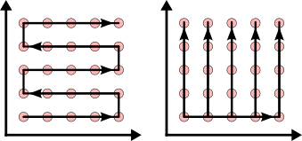
How to Process Data of Two or More dimensions

Since the ordering routine is only suitable for one dimensional data, the input data has to be rearranged if you want to treat problems of higher dimensionality.

We suggest two different approaches, which may be applied to an arbitrary number of dimensions:

Attention

Please always make sure that the ordering procedure was successful by plotting and checking the final molecular orbital overlaps and molecular orbital coefficients!